Robotics I

Poznan University of Technology, Institute of Robotics and Machine Intelligence

Laboratory 8 - Object tracking

Goals

By the end of this lab you will:

1. Understand how basic object tracking is performed
2. Wire up a Kalman-filter to trace the object motion
3. Forecast each object’s position into the future

Resources

• Extended Kalman Filter (EKF) on wikipedia
• Simple SORT overview (arXiv)
  
• Kalman Filter in OpenCV

Note: All code must run inside our provided Docker container.

Preparation

We are going to use the docker image used for classes 06 and 07.

Today’s class will not use ROS 2 to fully focus on the tracking aspects but the same logic can be implemented inside a ROS 2 node that was prepared during last week’s class.

To start we need to download the video that we are going to work today with:

1. Start/Attach to the docker container

2. Download the video

mkdir object_tracking && cd object_tracking && wget "https://chmura.put.poznan.pl/s/vsm7FpGL5r9weT3/download" -O video.mp4

Stage 1 - Run object tracking

0. It is needed to install the missing lap library for tracking in the Ultralitics framework:

pip3 install lap

Note: If the command fails (especially in Ubuntu 24.04), add the --break-system-packages flag to the command above.

Objective: Seeing the object tracks

1. We start with the modified Ultralytics object tracking exmaple that should be placed at the path /robotics1/object_tracking:

  # Python
from collections import defaultdict

import cv2
import numpy as np

from ultralytics import YOLO

# Load the YOLO11 model
model = YOLO("/robotics1/src/robotics_object_detection/weights/yolo11n.pt")

# Open the video file
video_path = "video.mp4"
cap = cv2.VideoCapture(video_path)

# Store the track history
track_history = defaultdict(lambda: [])

# Loop through the video frames
while cap.isOpened():
    # Read a frame from the video
    success, frame = cap.read()

    if success:
        # Run YOLO11 tracking on the frame, persisting tracks between frames
        result = model.track(frame, persist=True)[0]

        # Get the boxes and track IDs
        if result.boxes and result.boxes.id is not None:
            boxes = result.boxes.xywh.cpu()
            track_ids = result.boxes.id.int().cpu().tolist()
        else:
            pass

        # Visualize the result on the frame
        annotated_frame = result.plot()

        # Plot the tracks
        for box, track_id in zip(boxes, track_ids):
            x, y, w, h = box
            track = track_history[track_id]
            track.append((float(x), float(y)))  # x, y center point
            if len(track) > 30:  # retain 30 tracks for 30 frames
                track.pop(0)

            # Draw the tracking lines
            points = np.hstack(track).astype(np.int32).reshape((-1, 1, 2))
            cv2.polylines(annotated_frame, [points], isClosed=False, color=(230, 230, 230), thickness=10)

        # Display the annotated frame
        cv2.imshow("YOLO11 Tracking", annotated_frame)

        # Break the loop if 'q' is pressed
        if cv2.waitKey(1) & 0xFF == ord("q"):
            break
    else:
        # Break the loop if the end of the video is reached
        break

# Release the video capture object and close the display window
cap.release()
cv2.destroyAllWindows()

2. Run the script:

python3 tracking_example.py

3. You should see the video with white track following each detected object indicating where this object was previously seen. If you have issues then please check that:

• video file (video.mp4) and tracking script (tracking_exameple.py) where placed at the correct path (/robotics1/object_tracking)
• you have a yolo11n.pt model weight downloaded at the path (/robotics1/src/robotics_object_detection/weights/yolo11n.pt), which should have been completed during last classes
• you run xhost +local:root on the host machine if you just started a previously stopped container after system reboot.

Stage 2 - Understanding the tracking pipeline

When multiple detections appear in each frame, the core challenge is data association: deciding which detection in the new frame corresponds to previous set of image detections forming tracks for each object. A common pipeline combines:

1. Motion Prediction (e.g., via a Kalman Filter)
   
2. Similarity Computation (e.g., intersection‐over‐union between predicted and observed boxes)
   
3. Assignment (e.g., Hungarian algorithm)

A. Motion Prediction: Kalman Filter

• State: For each track, maintain a state vector
  \[ \mathbf{x} = [x, y, v_x, v_y]^\top \]
  where \((x, y)\) is the object’s center and \((v_x, v_y)\) its velocity in the image frame. Sometimes, we also store the bounding box size to also track the size of the detected object.
• Prediction: Project the state forward by one time step using the simple linear motion model
  \[ \mathbf{x}_{k|k-1} = F\,\mathbf{x}_{k-1|k-1} \]
  
• Update: When a detection is associated to that track (we see the same object in the new image), correct the predicted state: \[ \mathbf{x}_{k|k} = \mathbf{x}_{k|k-1} + K \bigl(z_k - H\,\mathbf{x}_{k|k-1}\bigr) \]

In popular SORT (Simple Online and Realtime Tracking) approaches, a constant‐velocity Kalman Filter predicts each track’s bounding box before matching.

B. Similarity Measure: Intersection over Union (IoU)

• For each predicted box (A) and detected box (B), compute
  \[ \mathrm{IoU}(A,B) = \frac{\mathrm{area}(A \cap B)}{\mathrm{area}(A \cup B)}. \]
  
• IoU values range from 0 (no overlap) to 1 (perfect overlap).
  
• Build a cost matrix (C) where
  \[ C_{i,j} = 1 - \mathrm{IoU}\bigl(\text{pred}_i,\,\text{det}_j\bigr). \]

C. Optimal Assignment: Hungarian Algorithm

• The Hungarian algorithm (Kuhn–Munkres) finds the minimum‐cost matching between two sets.
  
• Input: cost matrix (C).
  
• Output: assignment of track indices to detection indices that minimizes total cost (i.e., maximizes total IoU).
• As a result, we get the best matching between the previous tracks and the currently detected objects

Complete SORT Tracking Algorithm Workflow

1. Predict each existing track’s bounding box with the Kalman Filter.
   
2. Compute the IoU‐based cost matrix between predicted and detected boxes.
   
3. Assign tracks ↔︎ detections via the Hungarian algorithm.
   
4. Update matched tracks (Kalman filter update step).
   
5. Initialize new tracks for unmatched detections.
   
6. Delete tracks that haven’t been matched for a preset number of frames (“lost” tracks).

Provided YOLO tracking example performs all of the above steps, which resulted in white tracks drawn on the shown images.

Stage 3 - Future position prediction

Our objective today is to predict the future positions of the detected objects in the image based on current object positions and their history of motion. The goal is to draw our predictions as arrows starting from the center of the current detection pointing to the predicted position in 10 frames.

  # Python
#!/usr/bin/env python3

import cv2
import numpy as np
from ultralytics import YOLO

# Function to create a simple 4-state (x, y, dx, dy) Kalman filter
def create_kf():
    kf = cv2.KalmanFilter(4, 2)
    # State: [x, y, dx, dy]
    # Measurement: [x, y]
    kf.transitionMatrix = np.array([
        [1, 0, 1, 0],
        [0, 1, 0, 1],
        [0, 0, 1, 0],
        [0, 0, 0, 1]
    ], dtype=np.float32)
    kf.measurementMatrix = np.array([
        [1, 0, 0, 0],
        [0, 1, 0, 0]
    ], dtype=np.float32)
    # Tunable noise covariances
    kf.processNoiseCov = np.eye(4, dtype=np.float32) * 1e-2
    kf.measurementNoiseCov = np.eye(2, dtype=np.float32) * 1e-1
    kf.errorCovPost = np.eye(4, dtype=np.float32)
    return kf


def main():
    # Load the YOLO11 model
    model = YOLO("/robotics1/src/robotics_object_detection/weights/yolo11n.pt")

    # Open the video file
    cap = cv2.VideoCapture("video.mp4")

    # Dictionary to hold a KalmanFilter per track ID
    filters = {}

    while cap.isOpened():
        success, frame = cap.read()
        if not success:
            break

        # Run YOLO tracking to get stable track IDs
        result = model.track(frame, persist=True)[0]
        annotated = result.plot()  # draws bounding boxes + IDs

        # Extract center-based boxes (x, y, w, h) and track IDs
        if result.boxes and result.boxes.id is not None:
            boxes = result.boxes.xywh.cpu().numpy()  # shape (N,4)
            ids = result.boxes.id.int().cpu().tolist()
        else:
            boxes, ids = [], []
            
        # TODO: Predict the next state of all objects we are currently tracking

        # Update or initialize Kalman filter for each detection
        for (x, y, w, h), tid in zip(boxes, ids):
            
            # TODO: For each object we will have a separate Kalman filter. At this step either:
            # - create a new filter (there is create_kf() at the top)
            # - select a filter belonging to the currently analyzed object
            
            # TODO: Correct the filter state based on the measurement

            # TODO: Do the prediction of the state into the future: 10 steps, it has to be independent of on-going prediction/correction


            # Draw an arrow from current center to predicted center
            cv2.arrowedLine(
                annotated,
                # TODO: current position,
                # TODO: future position,
                color=(0, 255, 0),
                thickness=2,
                tipLength=0.3
            )

        # Display the frame
        cv2.imshow("YOLO + 10-frame Kalman Prediction", annotated)
        if cv2.waitKey(1) & 0xFF == ord('q'):
            break

    # Cleanup
    cap.release()
    cv2.destroyAllWindows()

if __name__ == "__main__":
    main()

The expected result should look similar to:

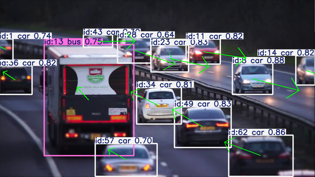
An example prediciton of a future object positions. Source: Own materials

💥 💥 💥 Assignment 💥 💥 💥

To pass the course, you need to upload the following file to the eKursy platform:

• a screenshot presenting the predicted positions of the objects in 10 frames into the future as arrows on the provided image